Ribbon Bar Command: Edit |

|

|
|
Ribbon Bar Command: Edit |
|
|
Ribbon Bar Command: Edit |
|
|
|
Ribbon Bar Command: Edit |
|
|
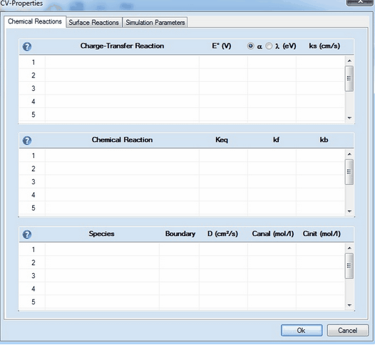
This command opens a CV-Property Dialog consisting of 3 property pages:
This page consists of 3 sections: •Charge Transfer Reaction •Chemical Reaction •Species
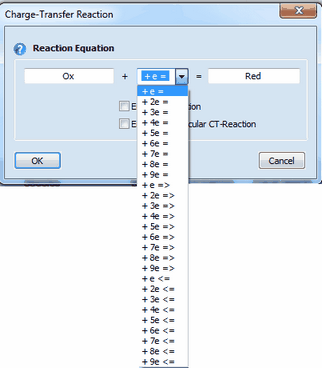
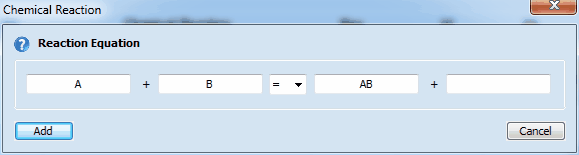
1. Adding a Charge-Transfer ReactionClick on the first empty line headlined Charge-Transfer Reaction. Enter the name of the species involved in the charge transfer process in the appearing dialog box
Syntax:
oxidized species + n e- = reduced species (kf and kb computed from Butler-Volmer or Marcus equation (the latter option applies only to n= 1)) oxidized species + n e- => reduced species (kb=0, kf computed from Butler-Volmer or Marcus equation the latter option applies only to n= 1) oxidized species + n e- <= reduced species (kf=0, kb computed from Butler-Volmer or Marcus equation the latter option applies only to n= 1)
Charge transfer reactions are always formulated to proceed as a reduction from the left to the right. Whether a charge transfer step does really proceed as reduction or oxidation is determined by the relation between initial and standard potential and the direction of the potential scan entered on the Property Page: Simulation Parameters and Chemical Reactions. •the species name of oxidized and reduced form must not be equal or empty •any character (including space) can be used in a species name but the first character must not be X, Y or Z •the number of electrons must be an integer ranging from 1 to 9
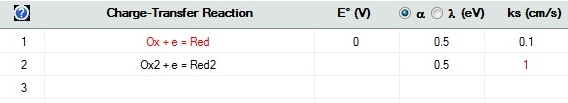
Checkbox: Enable AdsorptionActivate the Enable Adsorption checkbox if adsorption reactions need to be taken into account for the species involved in the underlying charge-transfer reaction. The adsorption parameters can be entered on the Property Page: Surface Reactions (see below) as soon as the input on the Property Page: Chemical Reactions has been completed. Note that E° and Keq must have been specified for each entered reaction and the required analytical concentrations must have been entered. Otherwise, access to the Property Page: Surface Reactions remains disabled. CT-Reactions involving adsorbed species are written in red as shown in the following picture:
Linking the heterogeneous rate constant of a CT reaction to the surface coverage of an adsorbed species. A heterogeneous rate constant, ks, written in red has been linked to the surface coverage of an adsorbed species. Click here for more details. Checkbox: Enable termolecular CT-Reaction
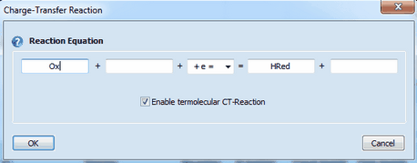
This enables the user to enter a termolecular charge transfer reaction (two species + electrode) of the following form
Ox + P + e = Red + Q
where P or Q might be an empty string as well. If both, P and Q are empty the CT-Reaction is treated as a "normal" bimolecular charge transfer.
Ox + H3O+ = HRed + H2O
have attracted increasing interest during the last couple of years.
2. Adding a Homogeneous Chemical ReactionClick on the first empty line headlined Chemical Reaction and enter the name of the involved species in the appearing dialog box:
Second-order chemical reactions comprising up to four species can be modeled: reversible reactions (Keq = kf/kb): Species1 + Species2 = Species3 + Species4
irreversible reactions (kb=0, independetly of Keq): Species1 + Species2 => Species3 + Species4 •if the name of a species starts with X, Y or Z it is considered a buffer/excess component. The concentration of such a species does not change in the course of the simulation •excess components or empty strings can be entered only for Species 2 and/or Species 4 •(pseudo-) first-order reaction: Species 2 and Species 4 are empty strings (or excess components) •second-order reaction: no species name or only the name of Species 2 or 4 is empty or that of an excess component
3. Editing or Removing a Reaction EquationReaction equations can be edited/removed simply by clicking on these reaction equation. The appearing dialog box provides the following options:
•Cancel •Copy Reaction •Remove Reaction •OK 4. Meaning of the Chemical/Electrochemical Parameters•Heterogeneous Reactions oEo (V), ks (cm/s) oButton α and λ (eV) •Homogeneous Reactions oKeq, kf, kb odepends on whether a first- or second-order chemical reaction has been entered.
5. Meaning of the Species Parameters•D (cm²/s) •Canal (mol/l), Cinit (mol/l) •Boundary
oBRB oORB
If electrode geometry is Spherical (Hg) the user has the choice to specify whether a particular species is forming an amalgam (i.e. diffusing into the mercury drop) or not.
|
||
|
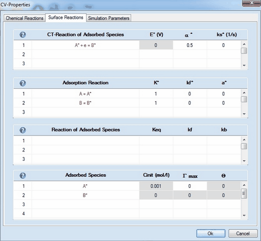
This Page can be entered only if •there is at least one CT-reaction for which the check box Enable Adsorption has been activated as shown above. •a value for E° (V) and Keq must have been entered for each charge-transfer and chemical reaction, respectively. •the required analytical concentrations, Canal (mol/l), of initially present species must have been entered. •the diffusion modus must not be Semi-Infinite 2D If only a single CT-reaction of the form Ox + e = Red has been entered on the Property Page: Chemical Reactions, the Property Page: Surface Reactions looks as follows:
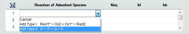
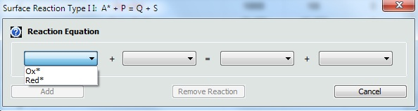
1. Defining a Reaction of Adsorbed SpeciesUnlike chemical reactions on the Property Page: Chemical Reactions, the definition of reactions between adsorbed and desorbed species is currently restricted to two predefined types: •Type 1: Red1* + Ox2 = Ox1* + Red2 •Type 2: A* + P = Q + S Click on the mouse button on the first empty line headlined Reaction of Adsorbed Species and select the reaction type from the appearing combo box.
Then use the combo boxes in the appearing dialog box to define the species involved in this reaction
2. Meaning of Parameters in CT-Reactions of Adsorbed SpeciesThe charge-transfer parameters in this section refer to the direct reduction of the adsorbed species. The latter are marked by an "*". •Eo* (V), ks* (1/s) •α* and λ (eV)* 3. Meaning of Parameters in Adsorption Reaction•K*, kf*
•α* 4. Meaning of Parameters in Reaction of Adsorbed Species•Keq, kf, kb
5. Meaning of Parameters in Adsorbed Species•Γ max •Θ
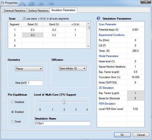
|
1. Scan Parameters:
•Scan segment, Estart (V), Eend (V), v (V/s)
•Check Box: use the same value of v(V/s) in each scan segment •Check Box: apply background correction •Potential steps (V) Removing scan segments:
2. Pre-Equilibrium•Disabled •Enabled •Smart
3. Diffusion•Semi-Infinite 1D •Finite 1D •Semi-Infinite 2D
4. GeometryDepending on the selected option for Diffusion the following geometry options are available
When selecting Spherical (Hg) the user has the choice to specify whether a particular species is going to form an amalgam (i.e. diffusing into the mercury drop) or not.
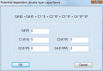
5. Experimental Conditions:•Ru (Ohm), Cdl (F) •Temp (K) 6. Model Parameters•Noise level (%) •Gauss-Newton-Iterations •Expansion Factor x-grid (perpendicular to electrode), Truncation error (%) oThe first one is a particular implementation of the box method which is the only simulation technique reported in the literature that yields exponential converges for the flux error towards zero when refining the grid expansion factor. The importance of the Expansion factor and the Relative truncation error for the accuracy of the simulated flux has been discussed in detail in a series of papers listed on the ElchSoft Homepage. The user is strongly advised to deal with these papers when working with DigiElch. Using the default setting for the Relative truncation error ensures that the flux error becomes independent of the selected grid expansion factor to the greatest possible extend. oThe second simulation technique implemented into DigiElch is an adaptive grid simulator. The starting grid is identical to that described above for the box method. However, the adaptive grid simulator does not result in exponential convergence for the simulated flux error. The error level originating from using an exponentially expanding space grid is therefore usually much larger than the truncation error. Consequently, the accuracy of the simulated flux can be guaranteed only when using a sufficiently small Local FEM Error (see more below). Also note that the adaptive grid simulator is not fully implemented. The following simulations cannot be executed with this tool: ▪simulation of two-dimensional diffusion systems ▪simulations involving amalgam forming species •Xmax / SQRT(Dt) 7. 2D-Simulations•Expansion factor y-grid (parallel to electrode) , Boxes for electrode 8. FEM- (Adaptive Grid-) Simulation•Local FEM Error 9. Level of Multi-Core CPU-Support•Level 0: •Level 1: •Level 2: •Level 3: •Level 4:
10. Simulation NameThere is a single-line edit control on the bottom of the Property Page: Simulation Parameters that can be used for giving the simulation a more meaningful name as that automatically generated by DigiElch. The name referring to the active simulation is indicated in the frame window of the simulation document after closing the CV-Properties Dialog. When exporting a simulation the default file name is either “simulation name.use” or “simulation name.txt ”. For this reason, the simulation name must not contain ‘\’ or any other character leading to problems in file names. |